

Inventory is more than stock on shelves – it is the physical representation of how a business plans, operates, and fulfils demand. It connects supply and production with customer service, while tying up a significant share of operating working capital.
This guide explains what inventory really is, how it behaves, and how to manage it with intent – linking Lean principles, Setpoint control, segmentation, forecasting, S&OP, and transactional insight into a coherent, practical framework for improving flow, service, and cash.
Inventory is where operations meet finance – a major driver of service, flow, and working capital.
Want to download this article for free?
Create a free account on My Academy Hub to download the article Inventory – Complete Guide, Metrics & Best Practices today.
Inventory is one of three core OWC levers
Together with Accounts Receivable and Accounts Payable, inventory determines how much capital is tied up in day-to-day operations – and how fast it turns back into cash.
Form, function, and purpose all matter
You can’t manage “inventory” as one number. Core types (RM, WIP, FG, GIT, MRO) and functional roles (cycle, safety, strategic, decoupling stock) each carry different risk, cost, and value.
The Setpoint defines “how much is right”
Optimal inventory is not a finance target, it’s an operational reality shaped by lead time, capacity, complexity, and predictability – and best calculated from transaction data, not opinions.
Safety Stock is insurance, not a hiding place
Well-designed Safety Stock reflects risk appetite and real variability. Poorly governed Safety Stock becomes a dumping ground for planning uncertainty and a silent drain on cash.
Techniques, segmentation, and policy must fit together
Reorder points, periodic review, JIT, and other methods only work when aligned with inventory segmentation (e.g. ABC/XYZ) and embedded into system parameters and governance.
Metrics need three lenses, not one
Financial (DIO, Turnover, GMROI), operational (WIP, SLOB, carrying cost), and service metrics (fill rate, stockouts, accuracy) must be read together. No single KPI tells the whole story.
Balance-sheet KPIs show the “what”; transactions show the “why”
DIO and GMROI reveal performance in aggregate; movement history, ageing, and order data show where flow breaks down – and where to intervene.
Most inventory problems are design problems
Bullwhip, SLOB, complexity creep and functional disconnects are symptoms of how the system is designed, governed, and incentivized – not just how warehouses are run.
Best practices are systemic, not tactical
Sustainable improvement comes from four disciplines working together: better forecasting, robust S&OP/IBP, intelligent inventory design (segmentation + suppliers), and data-driven governance.
Become a Certified Working Capital Expert with our accredited course Managing Working Capital
Inventory, together with Accounts Receivable (AR) and Accounts Payable (AP), forms one of the three core components of a company’s Operating Working Capital (OWC) – the capital tied up in day-to-day operations.
Among the three, inventory is the most tangible – and often the most complex – because it connects physical flow with financial performance.
Inventory is far more than “goods waiting to be sold.” Technically, it represents the cash invested in materials, components, and finished products that have not yet been converted into revenue.
How this complexity shows up depends on context.
Each environment defines inventory differently, but the underlying challenge is the same: aligning availability, cost, and cash.
And, while Accounts Receivable and Accounts Payable are strongly shaped by commercial and financial processes, inventory sits even closer to day-to-day operations.
Managing inventory is therefore a constant balance between efficiency (smooth turnaround and a strong return on Operating Working Capital) and effectiveness (ensuring availability to meet demand and service expectations) – and the quality of that balance determines both cash velocity and customer value.
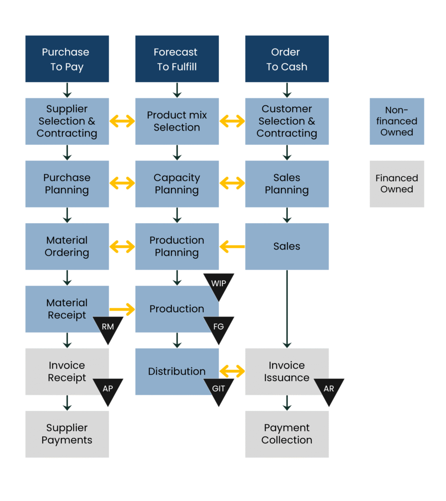
The Forecast to Fulfil (F2F) cycle describes the operational flow that translates demand signals – originating in the Order to Cash process – into material and production flow.
It spans production planning, material requirements planning (MRP), manufacturing, and delivery, defining how efficiently demand is converted into physical availability and customer fulfilment.
Inventory acts as both output and input in this process:
The Cash Conversion Cycle (CCC) describes the financial reflection of that same journey – how quickly cash invested in inventory is converted back into liquidity.
The Forecast to Fulfil cycle explains how inventory forms; the Cash Conversion Cycle explains how long it stays.
Effective inventory management therefore requires precise, connected decisions about:
Each choice directly affects both flow performance and financial return.
Inventory performance ultimately depends on how well the end-to-end flow connects – not only within operations, but across functions.
The Forecast-to-Fulfil process sits between two enterprise cycles:
When these streams operate in isolation, inventory becomes the shock absorber for their misalignment:
Effective operating working capital leadership therefore requires cross-functional collaboration between sales, operations, procurement, and finance to ensure that O2C, F2F, and P2P are synchronised.
Only then can inventory perform its true role: enabling flow, protecting service, and releasing cash.
When this cross-functional alignment is achieved, inventory shifts from a reactive buffer to an active performance lever.
All three elements of Operating Working Capital – Receivables, Payables, and Inventory – depend as much on operational behavior as on financial policy.
What distinguishes inventory is how deeply it is embedded in day-to-day execution. Its performance reflects how well the organization synchronizes planning, procurement, production, and logistics – not just how it measures financial outcomes.
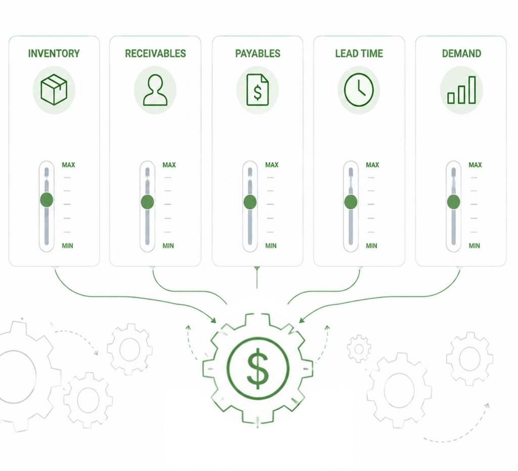
It responds to real constraints in the operating system – lead times, capacity, complexity, and predictability – the four defining boundaries of the Setpoint Framework.
These constraints establish what “good” looks like: the optimal level of stock required to maintain flow without unnecessary capital tie-up.
Knowing what “good” looks like enables you to read performance when it drifts off course – whether the business is carrying too much, too little, or the wrong type of inventory.
| Symptom | Likely Cause |
|---|---|
| Consistently high inventory levels | Overproduction, large batch sizes, poor flow visibility, or excessive safety buffers introduced to compensate for planning uncertainty. |
| Frequent stock fluctuations | Unstable planning cycles, poor demand signal quality, or weak coordination between sales, operations, and procurement. |
| Chronic shortages | Misaligned priorities, inadequate capacity flexibility, or reactive supply decisions that fail to match actual demand timing. |
Reading these signals correctly is critical for efficient inventory management.
In Lean thinking, inventory itself is classified as one of the Seven Types of Waste (Muda) – but it is also the consequence of the other six.
Reducing inventory sustainably therefore means stabilizing the process within its Setpoint, not forcing arbitrary cuts.
When managed this way, inventory becomes more than stock control – it evolves into a strategic capability that links cash efficiency with flow reliability.
Stable inventory practices support profitable growth, supply-chain resilience, and pricing power, while freeing capital for reinvestment.
In this guide, we explore inventory through that integrated lens of operating working capital, profitability, and operational excellence – connecting concepts such as the Bullwhip Effect, Slow-Moving and Obsolete Stock, the Setpoint Framework, and the Seven Wastes (Muda).
“Inventory doesn’t just reflect performance – it reveals it.”.

Technically, inventory represents goods and materials in various stages of production and movement.
To manage inventory effectively, it’s essential to understand what it consists of and how it behaves – across materials, processes, and locations.
The composition of inventory – what’s held, where, and why – defines both its operating working capital exposure and its strategic value:
To manage inventory deliberately, we first need to understand what it consists of – its forms, functions, and financial characteristics.
Each category of inventory represents a different point in both the value creation process and the cash conversion timeline.
How it is valued financially mirrors where it sits operationally – from raw material still waiting for transformation to finished goods ready to realise margin.
Together, these categories determine the shape of the total inventory: how long cash is tied up, how efficiently it turns, and how much risk the business carries between cost and sale.
| Core Type | Description | How It's Valued | Cash & Operational Impact |
|---|---|---|---|
| Raw Materials (RM) | Purchased components and inputs not yet used. | Material cost only (purchase price, freight, duties). | Capital tied up at the start of the cycle - before production adds value. Provides the greatest flexibility, as materials can be converted into multiple end-products. Levels are driven by supplier reliability, purchasing policy, as well as replenishment lead time and frequency. |
| Work In Progress (WIP) | Items in production or transformation. | Material + partial processing cost (labor, energy, overhead - often approximated at ~50% of total cost). | Capital tied up during value creation. High WIP signals flow inefficiency: e.g., bottlenecks, batching, or long cycle times that delay conversion to revenue. |
| Finished Goods (FG) | Completed products ready for sale or dispatch. | Full cost (material + complete processing + overhead). | Capital tied up after value has been added but before sale. Directly affects service performance and cash realization. Least flexible form of inventory - costly to hold, prone to obsolescence, discounting, and margin erosion if demand shifts. |
| Goods In Transit (GIT) | Inventory owned but in motion (shipping, transfer, or consolidation). | Material/Product cost + freight (if ownership transferred). | Capital tied up outside operational control. Fully consumes working capital but provides no immediate utility until received. High GIT often reflects long transport lanes or global sourcing complexity that lengthens the working capital cycle. |
| MRO & Spare Parts | Maintenance, repair, and operational (MRO) supplies not sold but required to run assets. | Replacement cost or acquisition cost (depending on accounting treatment). | Capital tied up in non-revenue-generating stock. Critical for asset uptime and continuity but prone to hidden accumulation and obsolescence. Often excluded from DIO metrics, yet significant for liquidity and operational risk if unmanaged. |
While core inventory categories describe what a company holds, functional perspectives explain why it holds them.
Each category serves a distinct operational purpose – from enabling flow and protecting against variability to supporting strategy and growth.
Understanding these motives is essential for optimizing inventory levels, managing risk, and balancing service with cash efficiency.
| Functional Category | Role & Purpose | Notes for Working Capital |
|---|---|---|
| Cycle Stock | Inventory consumed during normal operations between replenishments. | Baseline working inventory -determined by lead time and demand profile (typically: average weekly demand × lead time in weeks). Defines the minimum capital required to sustain normal flow. |
| Safety Stock | Statistical protection against forecast error and short-term demand variability. | Calculated using models that often consider required service level, demand variability, and lead time. Excess usually reflects unreliable planning or data. (See Section: Safety Stock and Risk Management for detailed methods.) |
| Strategic Stock | Inventory held intentionally beyond safety levels for business advantage: Risk Stock (supply disruption); Commercial Stock (promotions/launches); Price/Volume Leverage (MOQ or bulk discounts). | Governed choice, not error. Should be managed and reported separately to prevent it from becoming a permanent layer of inventory. Carries higher capital and obsolescence risk if not reviewed regularly. |
| Decoupling Stock | WIP buffers placed between process stages to maintain flow and protect throughput across bottlenecks. | Used to stabilise flow where processes are not perfectly synchronised. Essential around true constraints but excess often masks inefficiency or unreliable upstream performance. |
Understanding inventory by type and purpose is more than an accounting exercise – it’s a way to see how cash, risk, and operational behaviour connect.
Each category tells a story about how the business creates (or erodes) value:
Effective leaders view inventory not as static storage but as a strategic operating asset:
To perform this role, every inventory category must have a clear purpose, ownership, and governance model – anchored in its Setpoint:
This ensures that inventory levels are not arbitrary, but reflect the optimal point where flow, service, and capital efficiency coexist.
When managed at this level of intent, inventory becomes a designed capability – linking planning and execution to measurable financial outcomes.
Well-structured inventory transforms working capital from a by-product of operations into a designed capability – balancing service, resilience, and return.
You cannot optimize inventory you do not understand – and you cannot manage what you do not measure with intent.
Safety Stock sits at the intersection of service, stability, and working capital.
It is not a sign of inefficiency – it is an intentional buffer against the inherent variability in demand and supply.
But like any buffer, it must be measured, justified, and governed:
The art of Safety Stock lies in balancing risk appetite, forecast accuracy, and lead-time uncertainty – converting volatility into resilience without turning cash into comfort.

No forecast, supplier, or process is perfect.
Even in stable environments, variation occurs – customers order earlier, suppliers deliver later, production lines stop unexpectedly.
Safety Stock exists to absorb these shocks so that operations can continue uninterrupted while new stock arrives.
Its purpose is not to eliminate uncertainty but to prevent operational and customer service failure when uncertainty occurs.
When sized correctly, Safety Stock:
The level of Safety Stock therefore reflects a company’s risk posture – how much variability it is willing to absorb before service is affected.
There are several approaches to determining Safety Stock – ranging from simple rule-of-thumb calculations to advanced, system-driven models that continuously adjust for variability.
In this guide, we focus on the two most widely used and practical methods: a simple rule-based approach and a statistical (calculated) approach.
Both aim to define a buffer that protects service performance during the replenishment period, but they differ in precision, data needs, and governance complexity.
| Aspect | Simple Method | Statistical (Calculated) Method |
|---|---|---|
| Purpose | A straightforward rule using the difference between maximum and average demand and lead time to estimate buffer stock. | A data-driven approach that calculates the buffer needed to meet a chosen service level based on actual variability. |
| Formula | Safety Stock = (Max Daily Usage × Max Lead Time) − (Avg Daily Usage × Avg Lead Time) | Safety Stock = Z × σ₍d₎ × √L. Where: Z = Service-level factor (e.g. 1.65 for 95%, 2.33 for 99%); σ₍d₎ = Standard deviation of demand; L = Lead time. |
| When to use | Demand and lead times are stable; Data is limited; Simpler environments where ease of use outweighs precision. | Reliable demand and lead-time data exist; Volatility varies significantly by SKU; Organization seeks consistent, governed buffers |
| Advantages | Easy to understand and apply; Quick to calculate with minimal data; Suitable for early-stage control systems. | Reflects true variability and risk tolerance; Consistent across products and business units; > Aligns well with advanced planning tools. |
| Limitations | Can significantly over- or under-estimate needs when volatility is high; Does not explicitly separate demand vs lead time variability. | Requires accurate, maintained data; More complex to explain and govern; May fluctuate with statistical noise if not smoothed. |
Safety Stock should never be static.
It must evolve as forecast accuracy, supplier reliability, and demand variability change.
Left unreviewed, it drifts – either becoming an unnecessary comfort zone that absorbs cash or shrinking below the level needed to protect service.
Effective governance keeps it calibrated to both operational reality and business priorities.
Regular review – typically quarterly – ensures buffers remain aligned with actual performance, risk appetite, and service goals.
Best practices
A common pitfall is assuming that the service level used in the Safety Stock formula equals the service level achieved in practice.
In reality, realised performance often exceeds the modelled target, especially for stable or slow-moving items.
To maintain accuracy, companies should periodically compare realised vs. calculated service levels and adjust parameters or demand variability inputs accordingly.
At a strategic level, Safety Stock converts unpredictability into stability – but only when it is designed with intent and governed with discipline.
When treated as a governed asset rather than a blind cushion, Safety Stock strengthens both operational resilience and financial performance – turning variability from a threat into a managed, measurable component of sustainable flow.
Well-designed Safety Stock is not a comfort zone – it’s a control mechanism.
Inventory management techniques provide the mechanisms for replenishment and control, translating planning policies into day-to-day execution.
The method chosen depends on the nature of demand, supply stability, lead time, and operational complexity.
Selecting the right approach is key to balancing availability, efficiency, and working capital performance.
| Technique | Description | Best Used When | Working Capital Impact |
|---|---|---|---|
| Reorder Point (ROP) | Triggers replenishment when on-hand stock reaches a defined threshold. The reorder point is typically based on expected demand during lead time plus a safety stock buffer. | Demand and lead times are relatively stable, and continuous monitoring is feasible. | Keeps availability high without large buffers when parameters are accurate. Sensitive to forecast errors and data quality. |
| Periodic Review | Inventory levels are reviewed at fixed intervals, with orders placed to restore target levels. Between reviews, inventory is allowed to fluctuate. | Long lead-time items. Demand is predictable, and the cost of frequent monitoring outweighs the benefit of responsiveness. | Simplifies planning and administration but can lead to higher peaks and troughs in inventory levels between reviews. |
| Top-Off / Continuous Replenishment | Frequently replenishes high-turnover or fast-pick items during slow periods to ensure shelf availability during demand peaks. | Distribution and retail environments with high throughput and repetitive demand patterns. | Improves service and throughput with marginally higher average stock. Supports stable operations in high-frequency cycles. |
| Demand-Driven Replenishment | Reorders based on actual consumption or confirmed customer orders rather than forecasts. Often supported by integrated planning or pull-based systems. | Demand is visible in real time and supplier response is reliable. | Reduces overstock and obsolescence but increases exposure to demand spikes and supply delays if buffers are minimal. |
| Just-in-Time (JIT) | Aligns material deliveries and production schedules to minimise inventory holding. Materials arrive “as needed” for immediate use. | Supply chains are reliable, processes are stable, and demand is predictable. | Minimizes working capital and carrying cost but increases vulnerability to disruption or lead-time variability. |
There is no single “best” inventory management technique.
Each method represents a different balance between responsiveness, control, and capital efficiency – and should reflect product characteristics and demand behavior.
In practice, companies use a hybrid model:
Inventory techniques work only when governed as part of an integrated system that links:
Replenishment is not about restocking shelves – it’s about keeping cash, materials, and demand in motion.
Effective techniques allow the business to run not over-buffered, not starved, but stable, responsive, and financially efficient – turning inventory from a balancing act into a designed performance system where flow, cash, and service move as one.
Not all inventory should be managed the same way.
Segmentation provides the analytical foundation for differentiated control, allowing each inventory group to be governed according to its role, value, and variability.
By classifying items into segments – based on demand behavior, financial significance, and operational criticality – companies can apply the right management technique to each, rather than a one-size-fits-all policy.
Segmentation turns inventory management from a single target into a portfolio of Setpoints, each tuned to reflect its unique flow characteristics and cash exposure.
Inventory segmentation is the starting point for most Forecast to Fulfil (F2F) and operating working capital analyses.
Its significance and underlying principles are:
Different models can be used depending on industry, data maturity, and objectives.
Most organizations use one or more of the following frameworks:
| Model | Segmentation Basis | Application Focus |
|---|---|---|
| ABC / XYZ (Value / Variability) | Combines usage value (A–B–C) with demand variability (X–Y–Z). | A classic model for setting replenishment priorities and safety stock policies: e.g., A–X items tightly controlled, C–Z items managed more loosely. |
| Volume / Variability | Classifies items by sales or issue volume and demand volatility. | Determines which items benefit from make-to-stock vs. make-to-order or pull-based replenishment. |
| Volume / Coverage | Compares stock levels to demand coverage (e.g., days or weeks of supply). | Identifies overstocked or understocked items relative to consumption rate. |
| Value / Pick Rate | Cross-references item value with frequency of picks or issues. | Optimizes warehouse placement: high-value/low-pick items stored centrally; low-value/high-pick items located close to fulfilment points. |
You can’t manage all inventory equally – but you can manage it intelligently.
Implementation tip: Create segmentation models by location and inventory group (e.g., raw materials, finished goods, MRO). How you group inventory determines how it should be managed.
Strategic Conclusion
Effective inventory segmentation transforms policy into precision.
It ensures that effort, capital, and attention are focused where they create the most value – protecting flow where it matters, and releasing cash where it doesn’t.
Segmentation is therefore the bridge between strategy and execution:
When segmentation is embedded into planning and review, inventory stops being a uniform stock number – it becomes a structured, dynamic asset, managed differently by design to deliver consistent performance, service, and return.

Inventory metrics bridge finance and operations.
They translate movement and material flow into measurable financial performance – showing how effectively a business balances capital, cost, and service across its supply chain.
No single metric can capture the full story; each should be viewed in context with others to ensure balanced interpretation.
That’s why inventory performance is best understood through three complementary lenses – each addressing a different dimension of efficiency and effectiveness:
| KPI Level | Purpose | Typical Focus |
|---|---|---|
| Financial & Working Capital Metrics | Assess how efficiently inventory converts into cash and profit. | Working capital efficiency, liquidity, and return (e.g., DIO, Turnover, GMROI). |
| Operational Flow & Efficiency Metrics | Assess the internal effectiveness of processes - the speed, stability, and quality of flow through the value chain. | Process performance and waste reduction (e.g., WIP DIO, Obsolescence, Carrying Cost). |
| Service & Fulfilment Metrics | Evaluate how well inventory supports external effectiveness - meeting demand, protecting service, and enabling growth. | Fulfilment accuracy and responsiveness (e.g., Fill Rate, Stockouts, Inventory Accuracy). |
Together, these levels form an integrated performance framework:
Financial metrics translate inventory activity into balance sheet and P&L performance.
They reveal how effectively the company converts inventory into cash and profit, providing the foundation for liquidity and return analysis.
| Metric | Formula | What It Shows | Interpretation/Notes |
|---|---|---|---|
| Days Inventory Outstanding (DIO) | DIO = Average Inventory / COGS * 365 | Average number of days inventory is held before it is sold or used. | A core component of the Cash Conversion Cycle. Lower DIO improves liquidity, but aggressive reductions may damage service or resilience. |
| Inventory Turnover Ratio | Turnover = COGS / Average Inventory | How many times inventory is sold or used in a period. | Indicates speed of conversion from stock to cash. Low turnover = overstock; Very high = risk of stockouts. |
| Stock Cover / Days on Hand | Cover = Inventory / Average Daily Usage | How long current inventory will last at current consumption. | A forward-looking complement to DIO - operationally relevant. |
| Goods in Transit Ratio | GIT/Total Inventory * 100 | Proportion of inventory value tied up in transit. | Highlights structural inefficiencies such as long supply lines or global sourcing delays. |
Note on DIO Calculation:
While the standard DIO formula uses average inventory, the averaging method should match the reporting purpose.
In all cases, ensure COGS and inventory values represent the same time horizon and valuation basis.
A single DIO number can mask where capital and waste truly reside.
Breaking it down into Raw Materials (RM), Work-in-Progress (WIP), and Finished Goods (FG) provides diagnostic clarity – linking financial performance directly to operational flow.
| Aspect | Raw Materials | Work in Progress | Finished Goods |
|---|---|---|---|
| Formula | Average RM Inventory / Annual Material Consumption * 365 | Average WIP Inventory / (Material + 0,5* labor cost) * 365 | Average FG Inventory / COGS * 365 |
| Reveals | Efficiency of procurement and inbound flow. | Flow and throughput efficiency within production. | Balance between production and actual demand. |
| Typical Causes of Increase | Long supplier lead times, large order batches, high MOQs. | Bottlenecks, long setups, poor scheduling, or imbalance in process flow. | Overproduction, inaccurate forecasts, or long production runs. |
| Financial Impact | Early cash lock; higher working capital exposure. | Capital tied midstream without generating revenue; signals waste. | Obsolescence, markdowns, and gross margin erosion. |
Note on WIP DIO Calculation:
Decomposing DIO into Raw Materials, Work-in-Progress, and Finished Goods reveals where cash gets trapped, why it happens, and how to correct it.
Each component acts as a diagnostic lens on different stages of flow – from supply to production to demand.
Rising Raw Material DIO – Indicates inefficiency at the start of the cycle – where cash is committed before value is added.
Rising Work-in-Progress DIO – Signals friction within the flow itself.
Rising Finished Goods DIO – Exposes imbalance at the end of the cycle, where value has been created but not yet realized.
Viewed together, these trends trace directly to the Setpoint Framework:
Inventory efficiency is not measured by how little you hold, but by how effectively each unit of stock converts into margin and movement.
These metrics link operational performance with financial outcome – revealing whether inventory is working for the business or sitting idle as tied-up cash.
They expose three essential dynamics: profitability of stock, quality of flow, and cost of holding.
| Metric | Formula | What It Shows | Interpretation/Notes |
|---|---|---|---|
| Gross Margin Return on Inventory (GMROI) | GMROI = Gross Margin / Average Inventory Value | Gross margin earned per unit of inventory investment. | Links inventory to profitability. A GMROI > 1.0 means inventory is earning more than it costs to hold. |
| Profit per SKU / SKU Productivity | Gross Margin per SKU / Inventory Value per SKU | Identifies which products drive profit versus those that trap capital. | Supports SKU rationalization and portfolio optimization. |
| Obsolescence Ratio | Obsolete or Unsellable Stock / Total Inventory * 100 | Proportion of stock unlikely to sell at full value. | Indicates forecast error, poor design control, or ageing portfolio. Impacts both cash and margin. |
| Slow-Moving Inventory Ratio | Inventory Older Than X Days / Total Inventory * 100 | Portion of stock exceeding its expected turnover cycle. | Leading indicator for obsolescence and waste. |
| Inventory Carrying Cost % | Carrying Cost / Average Inventory * 100 | Annualized cost of holding stock (space, insurance, handling, financing). | Typically 20–30% per year; often underestimated when assessing working capital. |
Service & fulfilment metrics translate inventory performance into what customers actually experience – the ultimate measure of effectiveness.
They reveal whether stock is not only efficiently managed, but available when demand occurs – turning operational discipline into commercial reliability.
Balancing the two defines the true Setpoint: the level where cash, flow, and service performance are in equilibrium.
| Metric | Formula | What It Shows | Interpretation/Notes |
|---|---|---|---|
| Fill Rate / Order Fulfilment Rate | Orders Fulfilled On-Time and In-Full / Total Orders * 100 | Ability to meet demand directly from stock. | Directly influences sales and customer loyalty. Balance against DIO for optimal service. |
| Pick Rate / Line Efficiency | Order Lines Picked / Total Order Lines | Warehouse productivity and process flow. | Low pick rates reveal poor layout, inaccurate stock, or excess variety. |
| Stockout Frequency | Stockout Events / Total SKUs * 100 | Frequency of out-of-stock incidents. | High rates imply under-forecasting or overly lean policies. |
| Inventory Accuracy | System Quantity / Physical Quantity * 100 | Reliability of inventory records. | Foundational for trust in planning and reporting systems. |
Each of these measures connects customer experience to cash discipline. For example:
| KPI Symptom | What It Likely Means | Where To Look First |
|---|---|---|
| Low Fill Rate with High DIO | Inventory exists but not in the right place, form, or SKU mix. | Diagnose planning accuracy, inventory segmentation, and data governance. |
| Frequent Stockouts with Stable Demand | Replenishment logic or supplier reliability issues. | Review reorder triggers, lead-time assumptions, and planning cadence. |
| Falling Pick Rate and Rising Cost-to-Serve | Operational complexity or excessive SKU count. | Simplify flow, re-slot high-velocity items, or rationalize range. |
| Declining Inventory Accuracy | Signals a data-to-execution gap. | Even small misalignments cascade through DIO, service, and cash metrics. |
Together, these indicators help define the operational pulse of inventory management – how well the physical system delivers on the promises the financial system measures.
Financial KPIs like DIO, Turnover, or GMROI measure how inventory performs in aggregate – but they don’t explain why it performs that way.
They show the symptom, not the cause.
To truly manage inventory, organizations must look beyond static balance-sheet averages and analyze transaction-level data – the detailed movements, timings, and behaviors that define how flow actually operates day to day.
This is where operational truth becomes visible, and where the real levers for improvement lie.
Examples of inventory transaction data insights include:
| Focus Area | What Transactional Data Reveals | Why It Matters |
|---|---|---|
| Inventory Quality | Identifies Slow-Moving and Obsolete (SLOB) by SKU stock through last-movement or age analysis. | Enables targeted reduction of dead stock and frees cash for productive use. |
| Demand Patterns | Reveals seasonality, order frequency, and volatility by SKU, customer, or region. | Supports more accurate forecasting, segmentation, and safety-stock calibration. |
| Replenishment Efficiency | Measures purchase and production cycle times, reorder adherence, and supplier response. | Exposes structural drivers of high RM and FG DIO. |
| Pick and Fulfilment Rates | Tracks line-level execution: picks per order, on-time delivery, and fulfilment accuracy. | Connects operational flow to service reliability and working capital efficiency. |
Most balance-sheet metrics are averages – static snapshots over time.
Transactional data adds dimension, causality, and velocity.
It reveals how materials actually flow – how long they wait, where they accumulate, and where variability enters the system.
Together, financial and transactional analytics provide a 360° view of performance:
“Balance sheet KPIs tell you what happened. Transactional data tells you why – and what to do next.”
How Transactional Insight Links to the Setpoint
In a mature working capital system, transactional data is what keeps the Setpoint calibrated.
It transforms inventory control from a static reporting exercise into a dynamic feedback loop:
This integration creates a living control system – one where every decision on stock, replenishment, or service is grounded in evidence, not assumption.
When finance and operations interpret the same data through different lenses, they can jointly manage the trade-offs between service, risk, and cash – in real time.
Transactional visibility turns working capital from a quarterly ratio into a daily operating discipline.
Inventory performance is rarely the result of isolated decisions. It emerges from how a business designs its processes, manages variability, and aligns functions across the value chain.
The goal of this section is to address both the causes and the controls – connecting Lean waste elimination with Setpoint balance to achieve sustainable, high-performance inventory management.
In traditional Lean thinking, inventory is both a waste and a mask.
The goal of Lean is not “zero inventory” but smooth, predictable flow: the right material, in the right quantity, at the right time, moving seamlessly through the value chain.
What made Lean thinking revolutionary was its ability to give waste a vocabulary.
| Waste Type | Description | How It Affects Inventory |
|---|---|---|
| Overproduction | Producing more than is required or earlier than needed. | Creates surplus Finished Goods, inflates DIO, and increases obsolescence. |
| Waiting | Idle time when materials, machines, or people are waiting for the next step. | Leads to high WIP and low throughput. |
| Transport | Unnecessary movement of materials between locations. | Raises handling cost, increases GIT, and lengthens cycle time. |
| Motion | Excess movement of people or equipment during operations. | Reduces productivity, lowers pick rates, and raises cost-to-serve. |
| Overprocessing | Doing more work or adding features not valued by the customer. | Inflates cost and complexity, often increasing inventory of non-standard SKUs. |
| Inventory | Holding excess stock to compensate for poor flow or uncertainty. | Directly ties up working capital and hides upstream inefficiencies. |
| Defects | Errors or rework leading to scrap or quality issues. | Generates unusable or obsolete inventory and margin erosion. |
Each of the seven Lean wastes represents a design flaw in how the flow of materials, information, and decisions is structured.
These are not random disruptions but built-in inefficiencies: overproduction, waiting, motion, and other wastes are consequences of how the business is organised to plan, produce, and deliver.
Inventory is the visible footprint of invisible design flaws
When processes are overdesigned for efficiency, disconnected between functions, or driven by conflicting incentives, waste accumulates – and inventory rises to cover it.
From an inventory perspective, this relationship is direct and measurable:
These design-driven inefficiencies don’t create agility – they consume it.
Reducing waste therefore isn’t just about saving cost – it’s about restoring flow.
Every improvement in how processes are designed and sequenced – shorter setups, smaller batches, better synchronization – directly releases working capital and increases adaptability.
While Lean thinking identifies excess inventory as a waste, it does not by itself define how much inventory a business should hold.
This is where the Setpoint Framework becomes essential – translating Lean insight into operational balance by defining the optimal level of inventory that maintains flow without over-investing capital.
The Setpoint represents the equilibrium between service, flow, and capital – the level where inventory performs its intended function without masking inefficiency.
It is defined by four interrelated inherent supply chain conditions and constraints. These dimensions that determine how much inventory (and operating working capital) a company truly needs in order to operate efficiently and effectively:
| Setpoint Dimension | Description | How It Influences Inventory |
|---|---|---|
| Lead Time | The time between ordering and availability. | Longer lead times increase safety and strategic stock requirements; shorter lead times reduce DIO and improve agility. |
| Capacity | The ability of the system to produce or process. | Limited or rigid capacity forces larger batches and buffer stock; flexible capacity enables leaner inventory. |
| Complexity | The number of SKUs, process variants, and supply interfaces. | High complexity inflates cycle stock and obsolescence risk; simplification directly improves turnover and GMROI. |
| Predictability | The reliability of demand, supply, and process performance. | Low predictability drives safety stock and firefighting; improving forecast accuracy and supplier reliability stabilises flow. |
Together, Lean and Setpoint form a complete inventory management system:
The good news is that an Operating Working Capital Setpoint is not a matter of opinion or executive decree – it can be objectively calculated.
Unlike top-down targets pulled from the balance sheet, a true Setpoint is derived from transaction-level data that reflects how the business actually operates.
Setpoint turns inventory from a subjective target into an objective truth – measurable, operational, and real.
Want to learn more about the Setpoint Framework – including how to calculate it from your own transaction data? See our dedicated Setpoint guide.
Most organisations don’t struggle because their Lean systems malfunction – they struggle because those systems were never properly built in the first place.
Few companies have a shared understanding of what their optimal inventory Setpoint actually is, or how Lean flow principles translate into real operational control.
Without that foundation, the system reacts instead of regulates.
Each function – sales, operations, procurement, finance – makes local decisions that seem rational in isolation but collectively drive imbalance.
This is where recurring inventory challenges emerge:
These are not random market effects; they’re the external symptoms of internal design gaps – where Lean principles are absent and Setpoint discipline is undefined.
Even when Lean and Setpoint frameworks exist on paper, few supply chains behave exactly as designed.
Over time, small disconnects between planning logic, process design, and human behavior accumulate – creating larger distortions in flow, visibility, and capital efficiency.
The table below summarizes six recurring challenges that most organizations face – and how each one manifests in inventory performance.
Together, they form a diagnostic lens for identifying where process design, data quality, and decision behavior break down – and where to focus improvement to restore balance:
| Challenge | Cause / Description | Inventory Impact & Mitigation |
|---|---|---|
| 1. Bullwhip Effect – Amplified Demand Variability | Small fluctuations in end-customer demand become amplified upstream due to forecast distortion, order batching, and delayed or filtered data. Each tier reacts to perceived risk, inflating variability and inventory through the chain. | Impact: Excess FG and RM; long cycle times; inflated DIO. Mitigation: Shorten planning cycles; apply S&OP/IBP; share real-time demand data; reduce batching. |
| 2. Planning Assumption Drift – When System Parameters Age Out | Lead times, yields, MOQs, and cost assumptions are not updated as operational reality changes. Outdated system parameters create false precision in planning models and systematically bias safety stock and order quantities upward. | Impact: Mismatch between plan and reality; excess safety stock or shortages. Mitigation: Conduct quarterly parameter reviews in S&OP; use transactional data to recalibrate; assign clear ownership for master data accuracy. |
| 3. Forecast Misalignment & Visibility Gaps – Data Doesn’t Flow | Forecasts and demand signals are often created in silos, misaligned across functions, and disconnected from operational reality. Sales may forecast in value while operations plan in volume; finance may fix targets without synchronising timelines. Forecast ownership is unclear, horizons differ, and forecasts are treated as static numbers rather than living assumptions to be monitored and improved. | Impact: Overstock in low-visibility areas; shortages elsewhere; inflated buffers. Mitigation: Integrate forecasting with MRP/ERP; apply demand sensing; close feedback loops between planning and execution. |
| 4. Complexity Creep – Variety Outpaces Control | SKU proliferation, product customisation, and local variants multiply forecasting error, extend setup times, and increase obsolescence risk. Each variant adds administrative load and safety stock requirements, eroding turnover and agility. | Impact: Rising FG and component stock; slower turnover; SLOB exposure. Mitigation: Use ABC/XYZ segmentation; rationalize low-velocity SKUs; link product launches and phase-outs to inventory policy. |
| 5. Functional Disconnects – Local vs Global Optimization | Regional, functional, or departmental units pursue conflicting objectives - service, cost, or cash - without a shared framework for trade-offs. Local optimizations (e.g., purchasing in bulk for discounts or producing full batches for efficiency) improve individual KPIs but inflate total working capital | Impact: Stock imbalances across sites; duplicate safety stock; hidden transfers. Mitigation: Centralize visibility through IBP; define global vs local inventory targets; align ownership and accountability. |
| 6. Supply Chain Bias – Human Behavior That Inflates Inventory | Cognitive and behavioural biases (safety, hedging, legacy, incentive, technical) drive teams to add buffers or distort signals. Includes incentive bias, where local KPIs (cost, availability, quota) optimise one function at the expense of total working capital. | Impact: Persistent excess across RM, WIP, and FG; “comfort stock” masking underlying issues. Mitigation: Build awareness of bias patterns; challenge assumptions in S&OP; link KPIs to shared cash and service outcomes. |
Want to learn more about supply chain bias? Read our in-depth article on how behavioral patterns distort demand, planning, and inventory decisions.
The most visible long-term symptom of structural or process inefficiency is high levels of slow-moving and obsolete (SLOB) inventory.
While Lean waste and planning misalignment create the conditions, SLOB stock represents their financial consequence – materials and products that have lost velocity, value, or purpose.
Managing SLOBs effectively is therefore not only about cleanup; it’s about understanding how they formed in the first place – and preventing their return.
SLOBs are not just dormant assets:
| Category | Definition | Risk & Financial Impacy |
|---|---|---|
| Slow-Moving Stock | Items that have not turned within their expected cycle time (e.g. >90 or >180 days). | Early warning of imbalance between flow and demand. Ties up cash, raises carrying cost, and hides forecasting or setup inefficiencies. |
| Obsolete Stock | Items unlikely to sell or be used due to expiry, replacement, or design change. | Requires write-downs; directly erodes gross margin and occupies valuable space. |
Most SLOB inventory doesn’t come from deliberate overstocking – it results from design and behavioral issues elsewhere in the system. Over time, these combine to create a “residual layer” of dead stock – inventory that no longer serves the business but continues to consume resources.
SLOBs hurt profitability in three ways:
Effective SLOB management has two horizons: short-term recovery and long-term prevention.
SLOBs are the shadow of yesterday’s decisions – the cost of delay, indecision, and design drift.
When prevention and recovery are embedded into daily governance, SLOB management stops being a clean-up exercise and becomes part of continuous control.
The same principles that prevent stock ageing – visibility, ownership, and balanced flow – also underpin effective inventory design.
These form the foundation for the core principles and best practices that sustain long-term working capital performance.
Effective inventory management is not about one-off initiatives – it’s the result of disciplined design, alignment, and learning.
Sustained performance comes from how a company orchestrates the flow between demand, supply, and capital.
When these dimensions move in rhythm, inventory stops being a reactive buffer and becomes a designed capability – driving efficiency, service, and profitability.
The following best practices outline a proven framework for achieving that balance across industries.
1. Forecasting and Demand Alignment
Forecast accuracy is the foundation of inventory control.
Without it, planning and safety stock becomes guesswork, and DIO increases by default.
The goal is not perfect prediction – it’s predictable error that can be measured, monitored, and improved.
Best practices
Forecasts will always be wrong – the question is by how much, and how fast you know.
2. Integrated Planning and Decision Alignment (S&OP / IBP)
Sales & Operations Planning (S&OP) – or its advanced form, Integrated Business Planning (IBP) – connects commercial intent, operational capability, and financial outcomes.
It transforms inventory management from tactical firefighting into a strategic balancing act.
Best practices
S&OP is the control tower of working capital – where service, cost, and cash are synchronised.
3. Inventory Design and External Integration
No single inventory rule fits all products.
Segmentation and supplier collaboration enable differentiated control – aligning policy and practice with value, variability, and risk.
Best practices
Inventory efficiency is a network property – it depends on how information and trust flow across the chain.
4. Digital Control and Continuous Improvement
Optimisation is not a project – it’s a performance system.
Sustainable control depends on how well an organisation learns from its own transactions – not just from its reports.
The true measure of inventory health lies in the patterns of movement, not just the value on the balance sheet.
Modern governance links financial KPIs with transactional analytics to form a real-time feedback loop between cause and effect – showing not only what happened, but why.
Best practices
Inventory health lives in transactions – not in totals. Data-driven visibility turns working capital management from reporting into control.

Inventory is far more than stock on shelves – it is the physical expression of how your business actually runs. It reveals whether demand is understood, whether supply is synchronised, and whether decisions across sales, operations, procurement, and finance are working in harmony or pulling apart.
When these elements connect, inventory stops behaving like a reactive buffer and becomes a designed capability: protecting service, stabilizing flow, and releasing cash rather than consuming it.
The Working Capital Hub philosophy is simple:
Inventory excellence isn’t about having the lowest DIO — it’s about ensuring every unit of stock earns its place by enabling continuity, supporting growth, and strengthening return on capital.
When forecasting, planning, execution, and analytics operate as one coherent system, inventory becomes a strategic lever of performance — not a cost of doing business. That is the shift that distinguishes efficient organizations from truly resilient and profitable ones.


Take the course Masterclass – Managing Working Capital at the Hub’s learning center My Academy Hub and gain the skills to turn liquidity into growth and resilience.
